Our second project for Metis began with only two constraints:

1. Gather a substantial amount of data via web scraping
2. Build a linear regression model to attempt to predict a certain target

Being an aviation enthusiast of many years, I chose to look at a common complaint of many air travelers: delay. Would there perhaps be a way to predict, with any accuracy, the degree to which one might be late on a particular flight?

Approach

I decided to focus first on arrivals at one airport (ORD) from one origin (LGA) operated by one airline (American, quite arbitrarily), and expand from there if I had time. Canceled flights would not be considered. I would collect available arrival information, and calculate “lateness” by subtracting scheduled arrival from actual. This would be a simple measure of minutes, positive if late, and negative if early. Knowing the date would give me the day of the week. It was my hypothesis that some correlation might be found with lateness and both day of week and time of day. By using these features and others to build a linear regression model, I would see how much truth this held.

Scraping

Despite all of this information being available in a neatly-wrapped CSV file from the Bureau of Transportation Statistics, I decided to attempt to scrape data from one of the most popular flight data sites, which shall remain unnamed throughout this discussion. Sitting on a comprehensive trove of proprietary data, this site would much rather a user purchase their data than scrape it. Thus, they don’t make scraping a particualrly simple process.

As much of the data is posted via javascript, trying to read the page object generated using the requests module with Beautiful Soup is futile. By searching for a particular class value, one can navigate to the div containing the information of interest, but the div contains no text whatsoever.

Before giving up and changing tack, I decided to try Selenium, just in case there might be some luck to be had there. For whatever reason, the page source of the Selenium driver object did contain the desired data (in this case, all the relevant arrival times). Since each page is constructed live from the same template, it was fairly straightforward to use Beautiful Soup to extract the data from there.

Each flight number on each day had its own page, with the date, flight number, and a unique route number comprising elements of the URL. My scraping function looped through a list of flight number/route number tuples, advancing back into the year one day at a time, manufacturing a URL string to hand off to the webdriver for each day, until it was detected that there had been no flights for seven consecutive days. In this manner, I was able to collect nearly 2000 records for 17 different flight numbers for anywhere between two and seven months, depending on the flight number.

The biggest takeaways? First, scraping is an arduous process throughout which many, many things can and will go wrong. If one doesn’t properly anticipate within the scraping function how to deal with all these things (e.g. how to interpret a day on which a flight didn’t exist, what to do when the driver throws a timeout exception, etc.), it will not be uncommon to wake up in the morning to see that the function stalled out at 4am, halfway through the process, with none of the data saved. Which leads to the second but larger takeaway: work in batches and save often. In my case, I ended up putting code into the function that pickled the database every time a new flight number’s flights were added. It saved a whole lot of time in the end, and would have saved even more time had I done it from the beginning.

At some point, I would like to devote an entire post to the scraping process and the function used to make it happen, because it took some time to get it right, and there are a few things in it that I will do every time I scrape from here on out. But for now, onward.

Cleaning

Though the scraping process was somewhat arduous, the resulting raw data ended up being remarkably clean, and required very little to put it into useful condition. Here are the steps:

1. Convert all dates/times to datetime.
2. Add several new columns:
   • Lateness of gate arrival (minutes, actual gate arrival minus scheduled gate arrival) (Target)
   • Lateness of landing (minutes, actual landing minus scheduled landing)
   • Scheduled taxi time (minutes, scheduled gate arrival minus scheduled landing)
   • Day of week (0-6, by calling the .weekday() method on the scheduled arrival datetime objects)
   • Hour of day (0-23, by extracting the .hour attribute from scheduled arrival)
   • Quarter of day (0-3, simple chain of if-statements on hour of day)
3. Advance date for late-night arrivals — all datetime objects were stamped with the date on which the flight was scheduled to fly, so a 1am actual arrival would appear to have occurred nearly a full day before an 11pm scheduled arrival. When such impossibly-early lateness values were detected, the actual arrival times were rolled forward one day.
4. Drop records where scheduled taxi time < 0 — this indicated that the scheduled landing time came after the scheduled arrival time, a situation for which I had no concrete explanation.
5. Drop extremely late outliers.

To the latter, it was clear that my model was only going to be able to detect regular fluxuations due to trends of the schedule, and would have no ability to predict the extremes delays resulting from unpredictables such as weather, mechanical problems, air traffic control backups, etc. As such, I decided there needed to be some sort of threshold beyond which a record would not be used to train and test the model. For an idea of the distribution, here is a histogram of all lateness of gate arrival values:

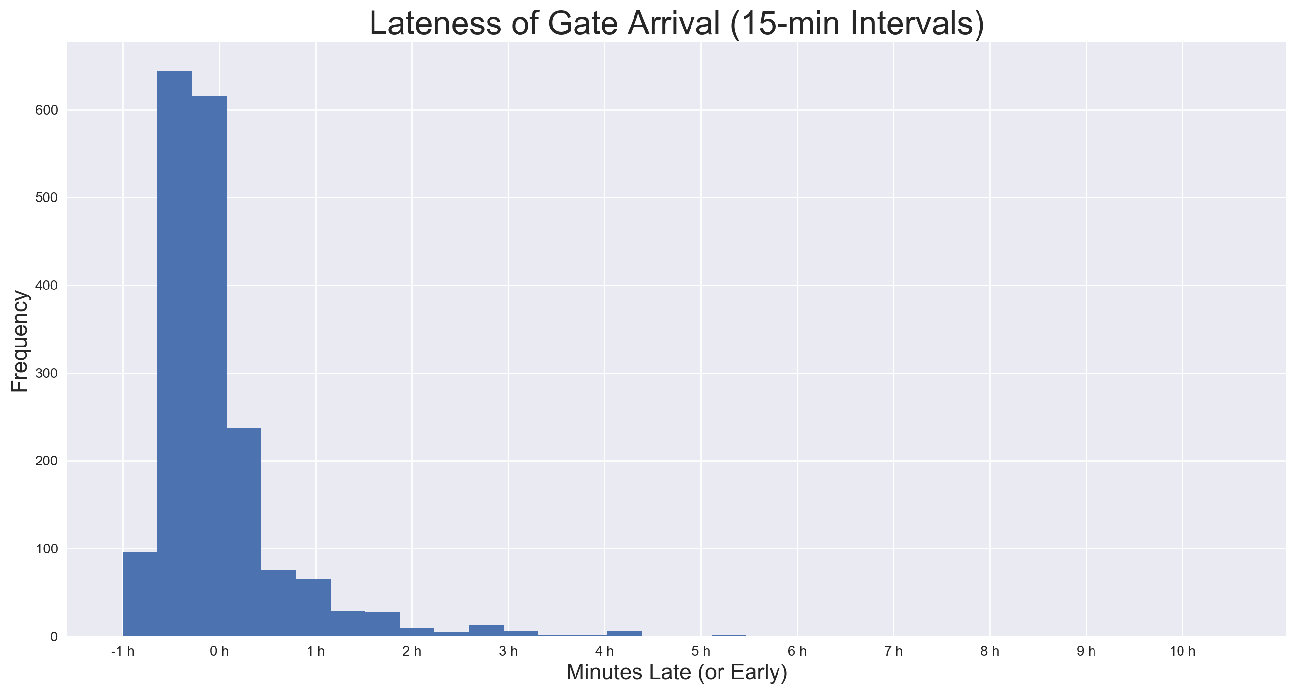
Here, it is clear that the vast majority of lateness values fall between -60 minutes and 60 minutes, with an ever decreasing number of values represented up until just over 10 hours (a very unfortunate flight indeed). I was surprised to see that the mode of the distribution falls below zero — indeed, most flights are early, with a median lateness of -12 minutes and a mean just under zero.

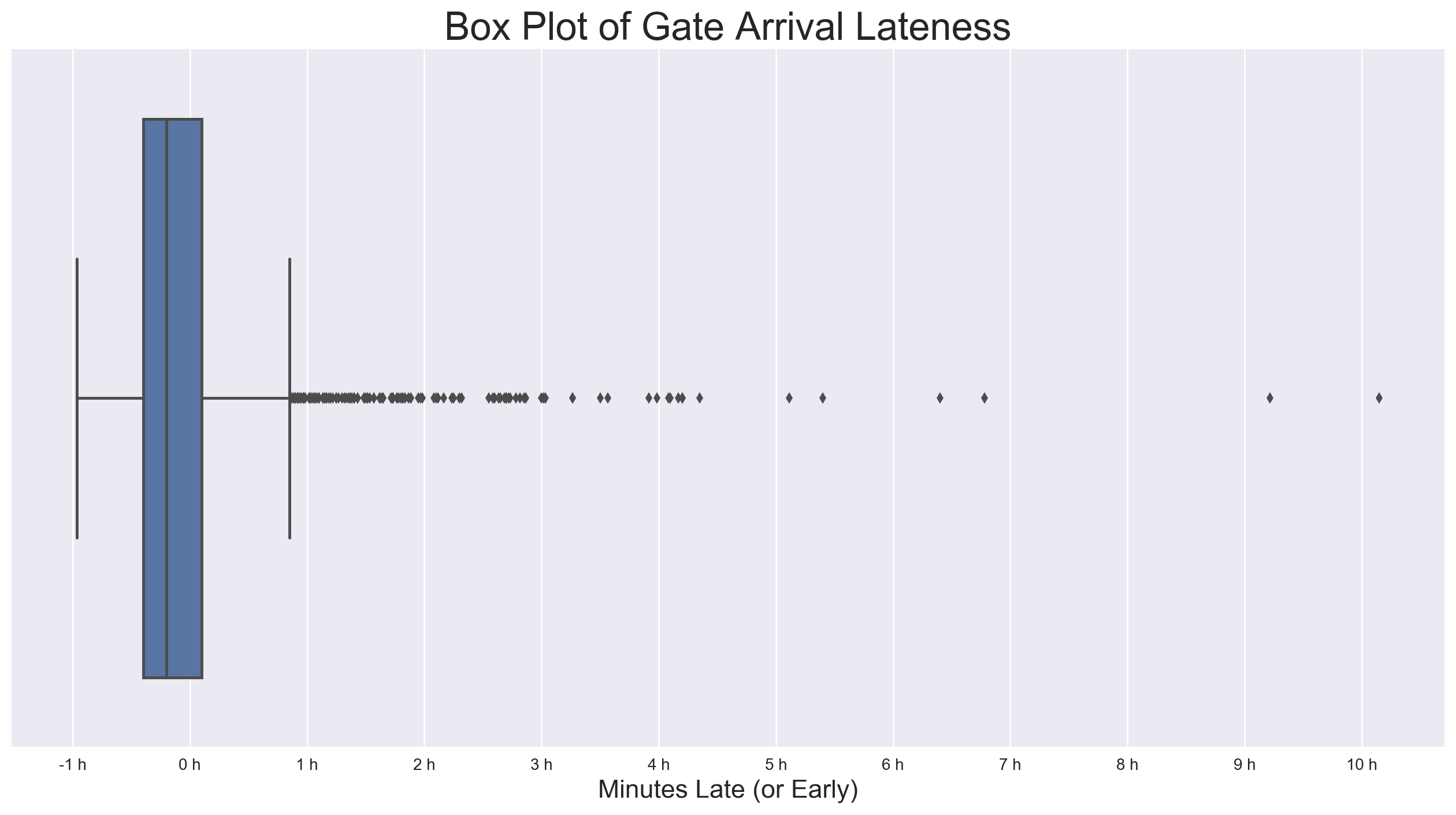
This box plot shows the distribution in a little more detail, and highlights the outliers beyond the upper whisker. At 1.5 times the IQR beyond the 3rd quartile, the lateness value here is 51 minutes. As it seemed arguable that any lateness values beyond this point would be caused by some sort of extreme and unpredictable event, I decided to use it as my threshold, and dropped records with lateness values in excess. Out of 1838 records, 153 had lateness values in excess of 51 minutes, or about 8.3%.

At this point, I also peeled off the final week of arrivals for use as a validation set after the model had been assembled.

Further Exploration

Given the task of selecting features that might have some power in predicting lateness, I chose to first look at lateness by day of week and time of day.

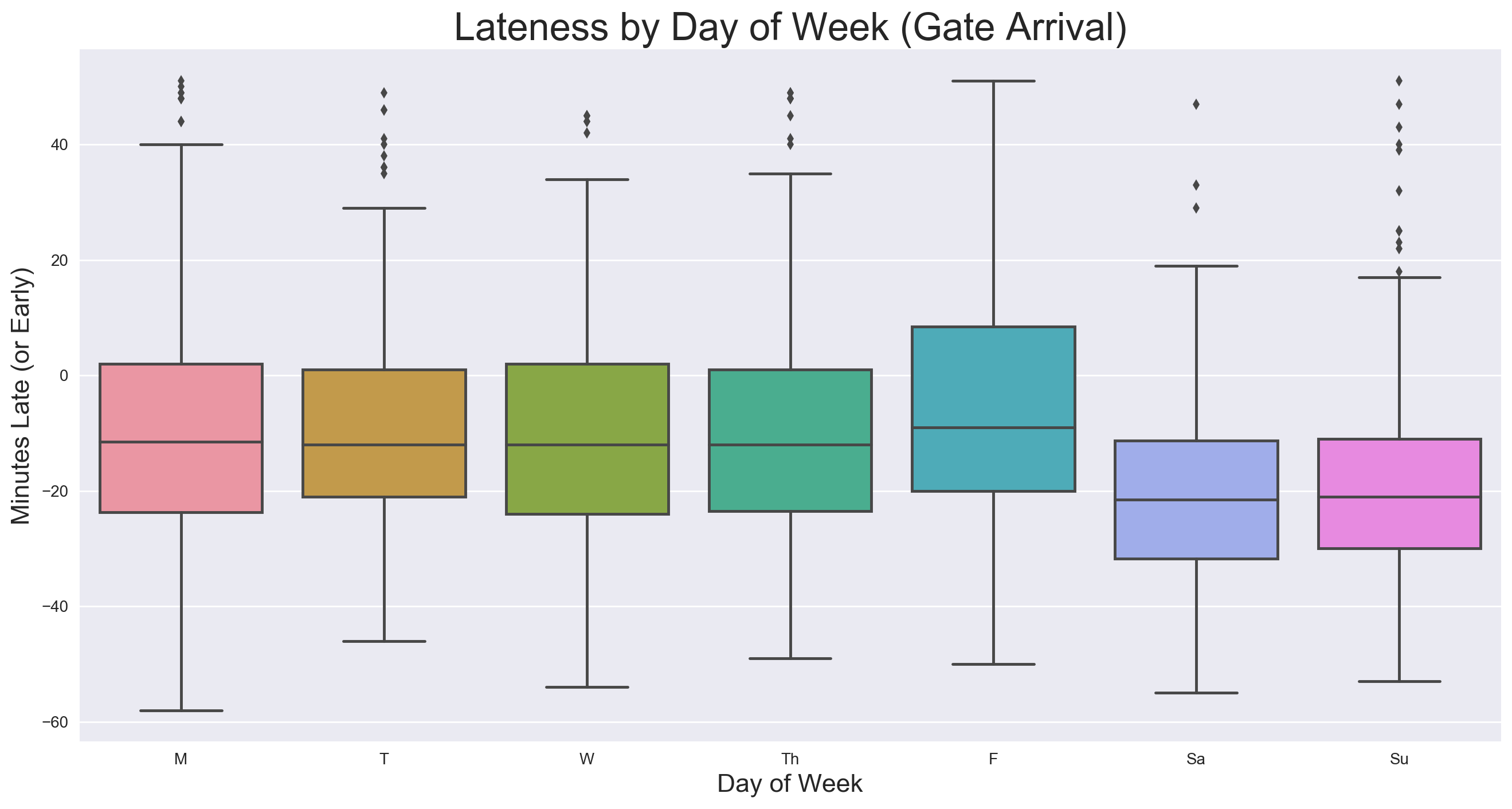
General variance appears to be similar from day to day. Median values on Monday through Thursday are almost identical, then Friday’s is a few minutes later, with Saturday’s and Sunday’s a few minutes earlier. Though there appears to be a slight trend, the median only varies within a 15 minute range, which is small considering the nearly 2-hour range of lateness values.

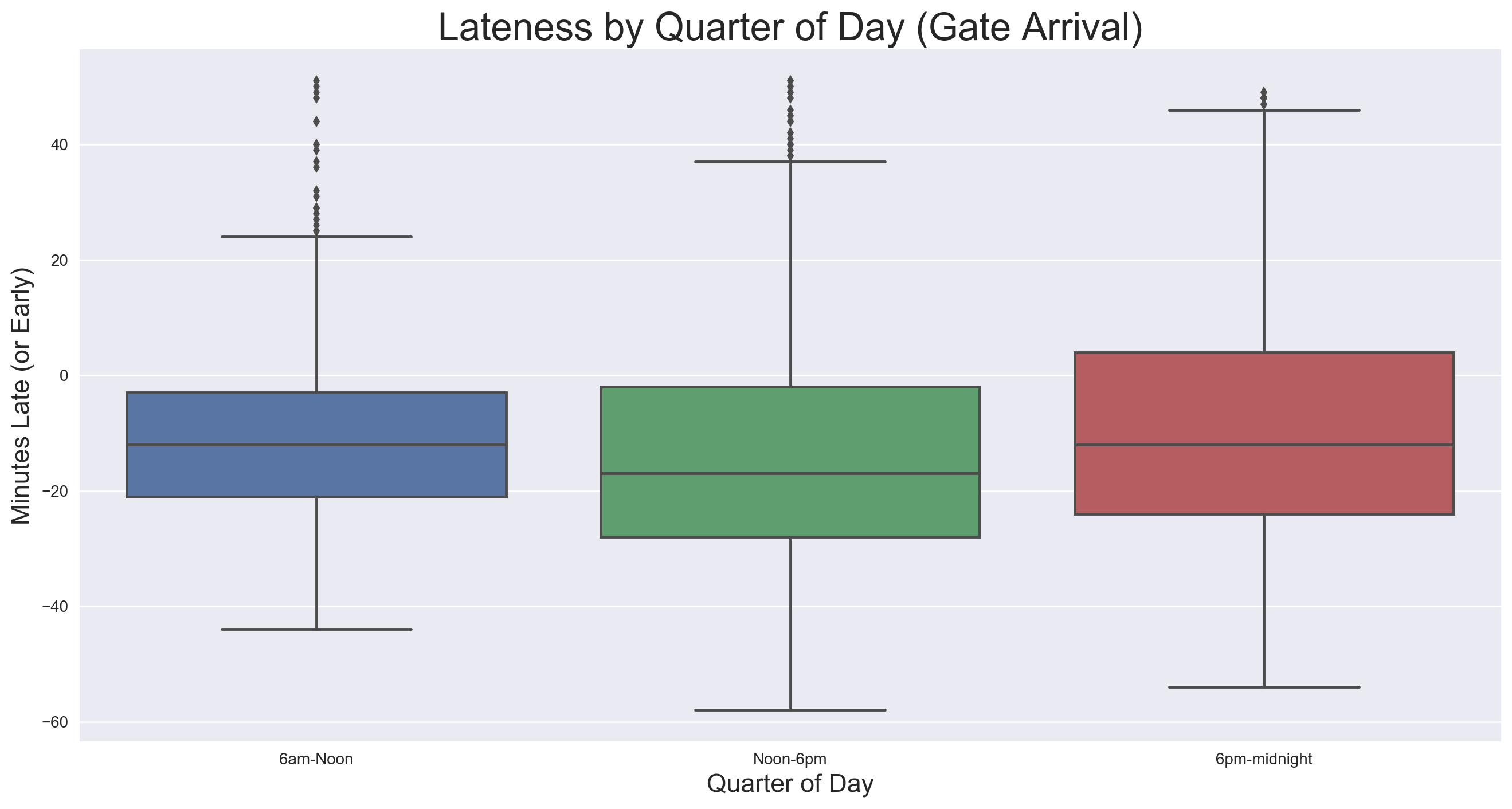
Because there are no flights scheduled to arrive between midnight and 6am, there are only three quarters displayed. There appears to be more variance as the day goes on, which intuitively makes sense, as irregularities in the schedule could compound throughout the day, widening the range come evening. The median doesn’t vary more than 10 minutes from quarter to quarter, with the afternoon being the earliest of the three.

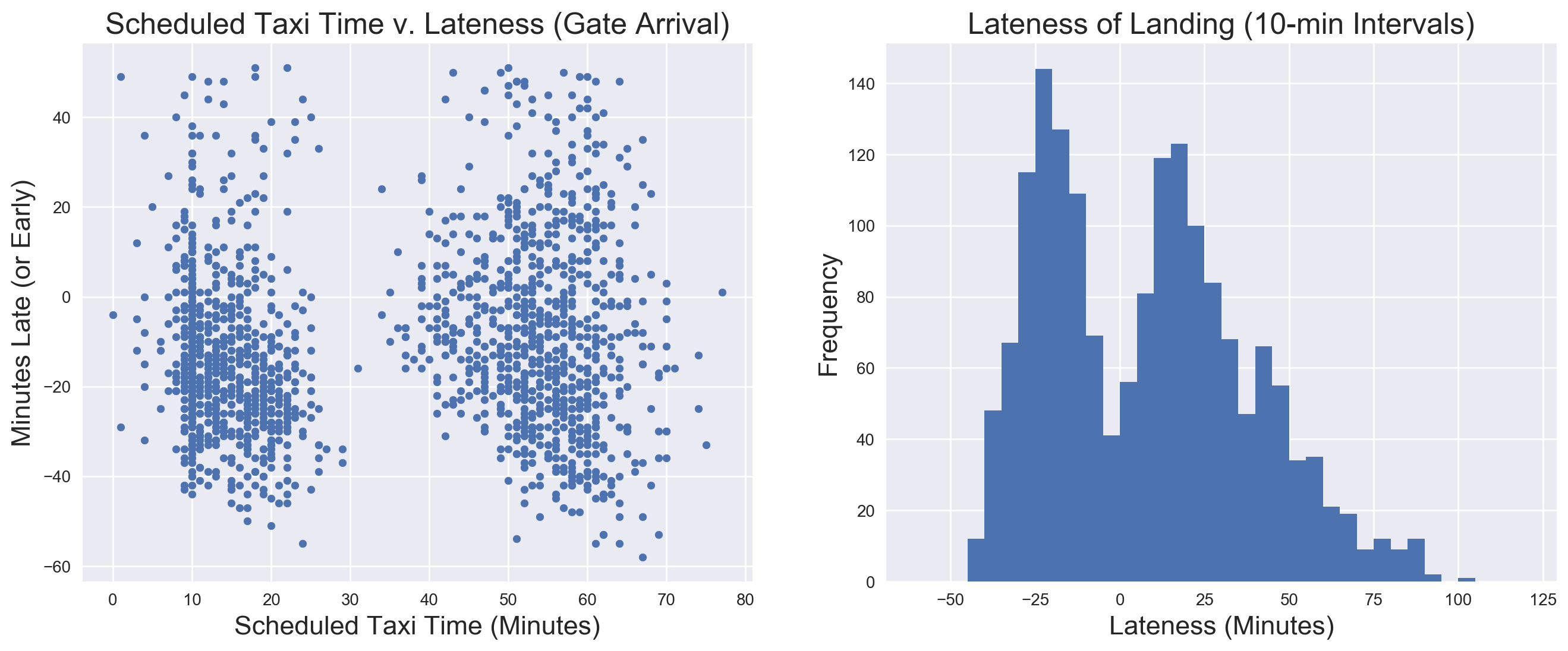
Scheduled taxi time remained the last feature for which I had any hope as a predictor, and the first plot on the left shows no obvious visual correlation with lateness of gate arrival. It is curious, though, that there would be two distinct groupings for scheduled taxi time (this is true for each day of the week). As lateness of landing (right plot) shows a similar bimodal distribution, and both were derived from the same arrival times, they are clearely related. At the time of writing, I have no explanation for this pattern, but will investigate further after the project has been completed.

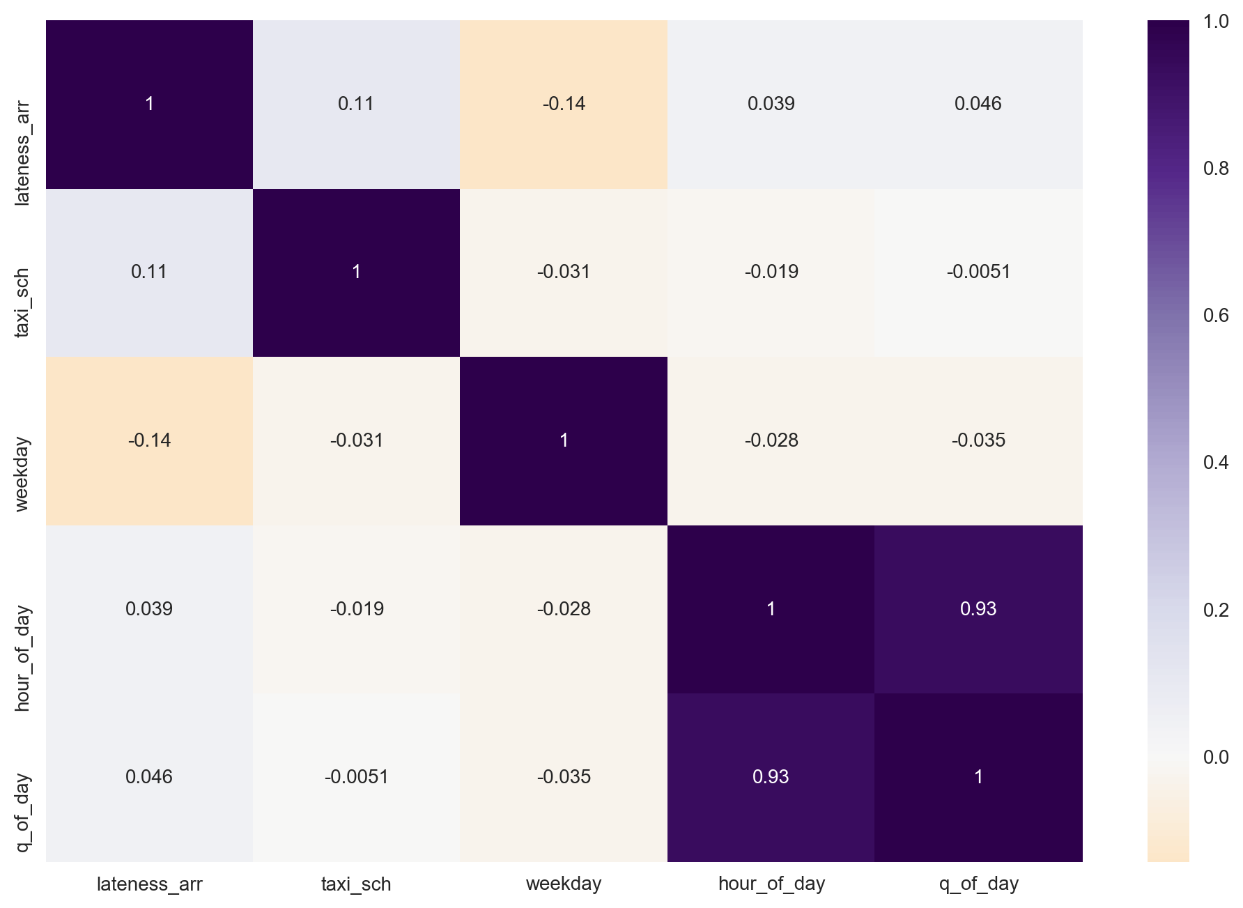
Looking at a heat map of correlations, there is very little evidence of correlation between any of the features and the target, the strongest magnitude being found with weekday (-0.14). Not surprisingly, quarter of day and hour of day show a great deal of colinearity, so it would likely be best to use one or the other when selecting possible features.

Linear Regression

In order to determine the best set of features for the linear regression model, I tried a quick test/train split on the full training set (20/80 of 1685 records), using the following combinations of features (and corresponding abbreviations):

• Weekday + Quarter of Day (WQ)
• Weekday + Hour of Day (WH)
• Scheduled Taxi Time + Weekday + Quarter of Day (TWQ)
• Scheduled Taxi Time + Weekday + Hour of Day (TWH)

None performed particuarly well, each with an RMSE_test (root mean squared error) around 19, and Adjusted-R² values ranging from 0.033 to 0.065. I chose to use RMSE here because I wanted to maintain the greater penalty for larger errors provided by MSE, but also keep the error in a meangful, interpretable unit — in this case, seconds.

To investigate each one further, I wrote a function to do a simple grid search, which performed a 5-fold cross-validation using each feature group, returning the RMSE for each fold as well as the mean RMSE for that round of CV. As with the trial round, no one model performed markedly better than any of the others, with the mean RMSE ranging between 19.27 and 19.51.

In this position, where no combination of features showed any predictive promise, scores all being grouped in a relatively tight and dismal range, it was incredibly difficult to argue that any one model was that much better than another and worthy of being sent to production. Were if a professional project of consequence, I would have gone back to square one in an attempt to collect other features that might show a stronger correlation with lateness. But for the sake of exercise, I chose to use the feature set with the lowest RMSE, TWH, despite its second-place Adjusted-R² value of 0.057.

To establish a baseline RMSE, I used the SciKit-Learn DummyRegressor() model, which simply takes the mean of the training set targets and predicts that value for every case. This method yielded an RMSE of 15.26.

After training the final regression model on the full training set (using the TWH features), I used it to predict on the reserved test set. Not surprisingly, a plot of predicted lateness versus actual does not show any clear evidence of predictive power, as the points would gather around the red line were it present:

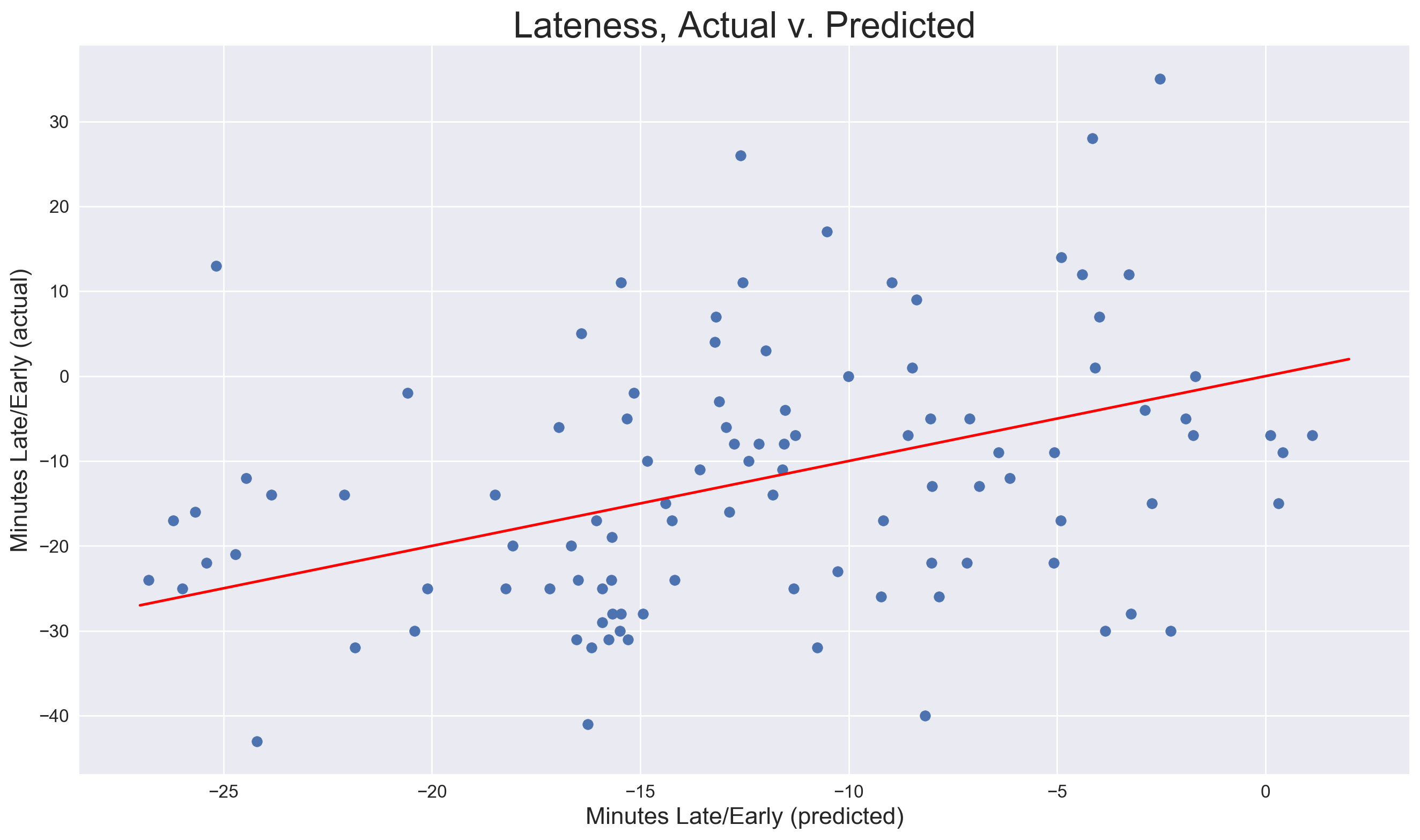
This was further confirmed by an RMSE of 14.51, which, though nearly 5 seconds below the cross-validation RMSE, would ideally be much closer to zero. However, the fact that it beats the dummy regressor’s RMSE by 0.74 suggests the faintest presence of predictive power.

Conclusion

Though more schedule-derived features may help to eke out a touch more accuracy (e.g. take-off information, which I failed to include in my first round of scraping), it is my sense that scheduling information would never be sufficient to reliably predict how late or early a flight might be, as the point of scheduling is to provide a framework in which operations can run smoothly. After this exploration, I have no doubt that the airlines have largely figured out optimal arrival and departure times based on a weekly and daily ebb/flow of traffic, and other such periodic trends. If a flight scheduled to arrive at 6:00pm on Friday is consistently 15 minutes late, just schedule it to arrive at 6:15pm instead. I would be curious to plot scheduled gate-to-gate times for flights along the same route, day to day, hour to hour, as I suspect this would reveal an accounting for traffic flows.

Beyond scheduling information, predicting lateness comes down to predicting such things as the weather, mechanical failures, natural disasters, and human error. Some may be decently predictable in the short term, and the probability of others can be greatly minimized. But trying to accurately predict that particular flight will be two hours late some days ahead of time essentially comes down a coin toss — using a coin that many would describe as quite unfair.