For our first project here at Metis, we were asked to respond to an informal RFP from a fictitious non-profit of the name Women Tech Women Yes, which solicited analytics advice to guide the placement of their promotional street teams in advance of their annual fundraising gala. As street teams would be placed at the entrances of subway stations to collect email addresses in exchange for free tickets to the gala, they suggested using the freely-available MTA data to determine which subway stations might be the most beneficial to target. The stated interest was in collecting as many signatures as possible from “…those who will attend the gala and contribute to our cause.” No specific date for the gala was given, though they mentioned it would be in early summer.

Approach

Given a designation of “early summer” for the time of the gala, we decided to analyze turnstile data for the five weeks spanning the month of May in 2016, given that this would be the prime promotional period for an event in June or July.

Our potential client stated that they were looking not only for enthusiastic attendees, but for those who might have the resources and the inclination to donate to the cause. This being the case, we decided to determine the busiest stations in proximity to 50 prominent NYC tech companies and 10 universities, and recommend that these be targeted for promotional efforts. Our list of companies was determined largely by finding the largest employers in the sector, and the list of colleges by prestige.

We decided to use the total traffic per station over the duration of the dataset to rank the busiest stations, as opposed to doing any timeseries analysis and breaking it down per day or per time of day. Surely some insights could be gained by this approach, but the assumption was that we wouldn’t get any great surprises by looking at slices, and that after work would be the best time to catch people regardless. We also found it a better use of time to focus on determining station proximity to relevant businesses and colleges.

To that end, we employed the Google Maps API to pinpoint the exact location (latitude and longitude) of all MTA stations, businesses, and colleges. We then gave each station a weight based on its proximity to these businesses and companies, and used that weight along with its total traffic to determine the overall relevance score of that station. Finally, we ranked stations by their relevance, and the top stations on this list were the ones we recommended to the client as the best to cover with their street teams.

Exploratory Analysis and Cleaning

Though the MTA dataset appeared to be remarkably clean, there were a handful of challenges that had to be addressed before we could arrive at any meaningful calculation of total station traffic. Those I will address here include how best to sort the data, what constitutes a unique station and how exactly to determine that, and how best to filter out invalid traffic measurements.

For reference, here are several sample rows of the raw turnstile data upon loading into pandas:

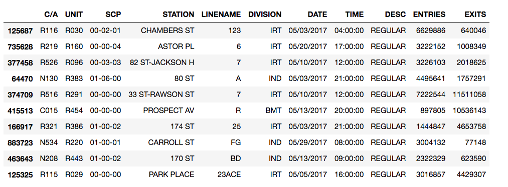
The period between readings is generally four hours, occuring regularly on the 4s, 8s, and 12s, though there are occasional exceptions.

Unique Stations

STATION does not provide a unique station ID. For example, of all the unique values in the STATION column, only one contains 23 ST, implying that there would only be one 23rd Street station. This is one of the many times where I was thankful for my 14 years of NYC residency, as there are five stations of that name: one for each of the CE, 1, FM, NRW, and 6 trains. We would need to go beyond STATION to find a unique identifier.

Grouping by STATION and then LINE largely took care of this problem. The five 23rd St stations were grouped properly, as were others with redundant street names. Instead of relying only on groupby throughout, we merged STATION and LINE to form another column, UNIQUE_STATION, and then filtered out STATION and LINE in the process, as we did not foresee needing to use them on their own.

One thing we noticed was that several of the larger stations were broken up into two or more component stations. We considered merging these as well, but decided to uphold the convention, as the separation is real and geographic in some cases. Take 34th St Penn Station, for example. One portion, 34 ST-PENN STA - ACE, represents the entrances on 8th Avenue unique to the ACE line. Another, 34 ST-PENN STA - 123, represents those on 7th Avenue serving the 123 line, and the final, 34 ST-PENN STA - 123ACE, represents the entrances from either station to Penn Station itself.

As these can be as much as one long block apart (~0.25 mi) and serve entirely different lines, it makes sense to preserve their independence.

Sorting

What are C/As? Units? SCPs? And how do they relate to stations?

According to the Field Descriptions file available on the MTA developers page, C/A = Control Area, UNIT = Remote Unit, and SCP = Subunit Channel Position, which represents a specific address for a device. But there’s no great indication of exactly what Control Areas or Remote Units are, or how they relate to stations or SCPs.

By a series of groupby adventures, one can finally figure out the following hierarchy:

• Remote Unit — Usually one per stations, one Remote Unit can sometimes cover two small stations, while a larger station may encapsulate two
• Control Area — A subdivision of a particular station
• Subunit Channel Position — The atomic unit of this data set: the individual turnstile. SCPs are grouped within Control Areas.

SCPs do not have unique identifying numbers within the MTA system, or even stations, only within their C/A. Thus, one cannot simply sort by SCP to get continuous streams of data from each turnstile, as each could be interspersed with others of the same number. To observe a stream of uninterrupted data for each turnstile, we sorted by the following hierarchy:

UNIQUE_STATION > UNIT > C/A > SCP > DATE > TIME

Filtering

In theory, calculating the difference between one cell in ENTRIES or EXITS and the previous theoretically yields the total number of people through the gate during the period between readings. With reliable figures, one could simply sum these values for each station and add entrances and exits together to get the total traffic of that station.

Creating the differential columns takes no more than a couple lines of code:

may_df['ENT DIFF'] = may_df['ENTRIES'].diff()
may_df['EX DIFF'] = may_df['EXITS'].diff()

Exploring the range of values in the resultant DIFF columns reveals a spread from roughly -1B to 1B, indicating the presece of more than a few numbers that couldn’t feasibly represent people moving through a single turnstile, as we would expect a range of values between 0 and a few thousand. Several cases explain these anomailes.

When we reach the end of one turnstile’s count and continue with the next (switch from one SCP or C/A to another), the differnential does not represent an actual count. Occasionally, a turnstile is reset or replaced. In the first case the differential will be a negative number, and in the second case the differential could be negative or positive. In either case, the differential will almost always be several orders of magnitude larger than the largest feasible entry or exit count, and will not represent actual people passing through the gate.

Some turnstiles count backwards, so the differential between current and previous cells in ENTRIES or EXITS will be a negative number in those cases, but the absolute value of this number represents a genuine count. Another case in which negative numbers appear is that in which several readings from a different turnstile are mislabeled with the current turnstile’s SCP number and mixed into the series. This generates alternating negative and positive differentials.

Correcting for a switch from one turnstile to another is not a difficult fix; whenever a new C/A or SCP value is detected, we set the DIFF columns to zero:

may_df.loc[(may_df['SCP'] != may_df['SCP'].shift(+1)) |
           (may_df['C/A'] != may_df['C/A'].shift(+1)),
           ['ENT DIFF', 'EX DIFF']] = 0.0

This gets rid of a lot of the bogus values in the ±(1E4-1E10) range, though a histogram of the absolute values of both DIFF columns shows plenty of anomalies due to the other cases (y-axis on log scale):

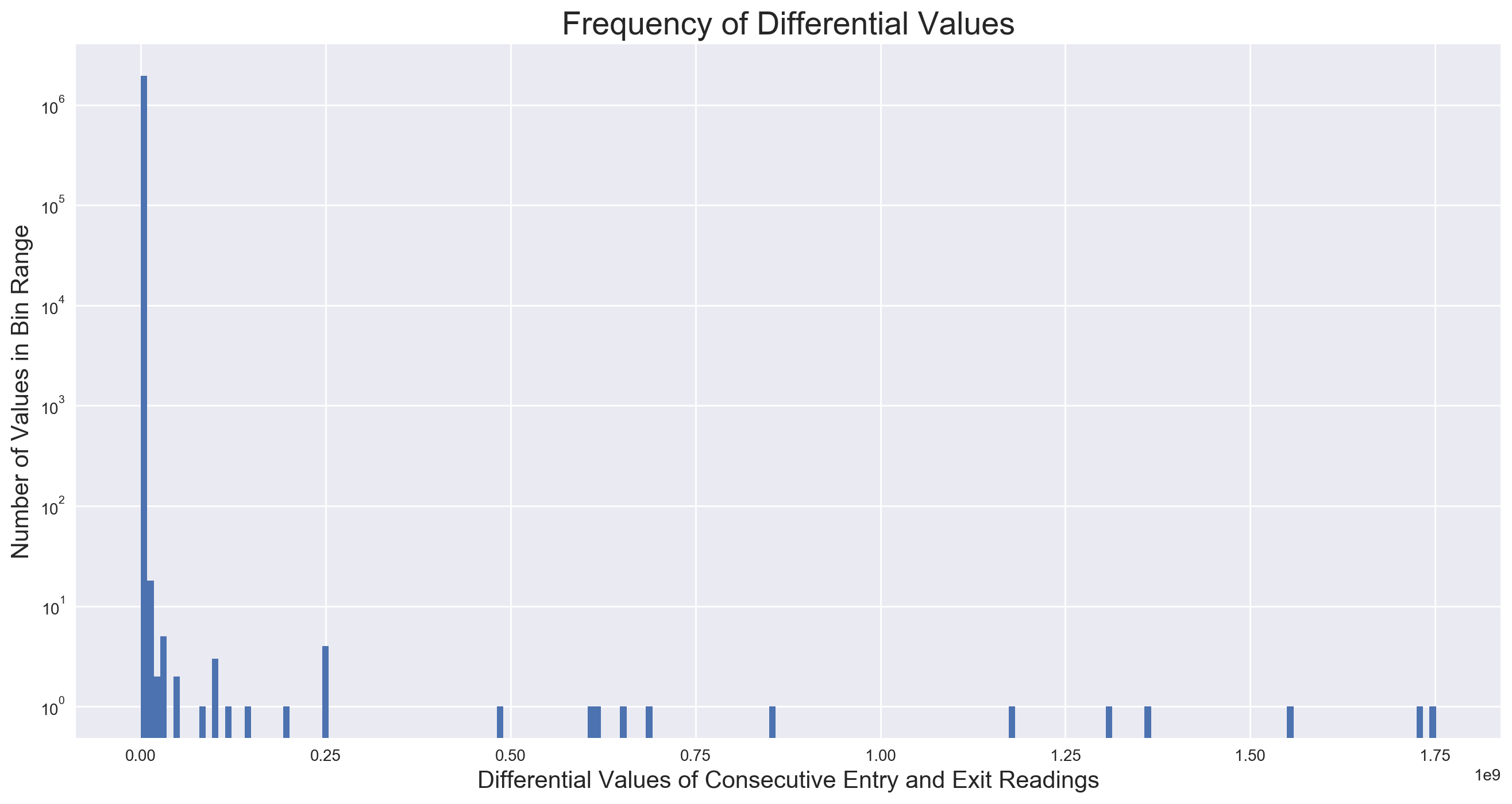
The values we want to keep are all or almost entirely contained within the first bin on the far left, of which there are about a million more than there are of any other value range. How best to filter? In order to inspect the right “neighborhood” of entry and exit differentials to determine the best filter value(s), we try to determine a realistic maximum number of people that could flow through a single turnstile during the observational period of four hours. One swipe every four seconds seems to be a realistic estimation, which yields 900 per hour, or 3600 per four hours.

Inspecting negative values with an absolute value in this range, we fing that almost every instance of a differential between -3000 and 0 represents a valid reading by a backwards-counting turnstile, and every instance less than -3000 is a bogus value as a result of cases described above. However, an inspection of the positives reveals legitimate counts as high as the 4000s, and another special case: a turnstile going offline from anywhere from a few hours to a few days, then coming back online and dumping all the counts for the duration of the offline period. As we are concerned with the total traffic over the duration of the data, these counts could be considered legitimate, and we elect to keep them. Thus, we filter any values in the DIFF columns less than -3000 or greater than 8000.

Note: I learned a valuable lesson here about when to roll up the sleeves and put in some hours, and when to take a shortcut. Turns out, using the our estimated max number of people through a turnstile over four hours as a filter threshold, 3600, returns the same results as our more specific and more accurate -3000 and 8000 cutoffs. I easily spent 4-6 hours digging through values in that range, trying to figure out the best threshold(s) and what all the exceptional cases were. And while this was fun, that time could have been much-better spent on all sorts of other things. For the next time.

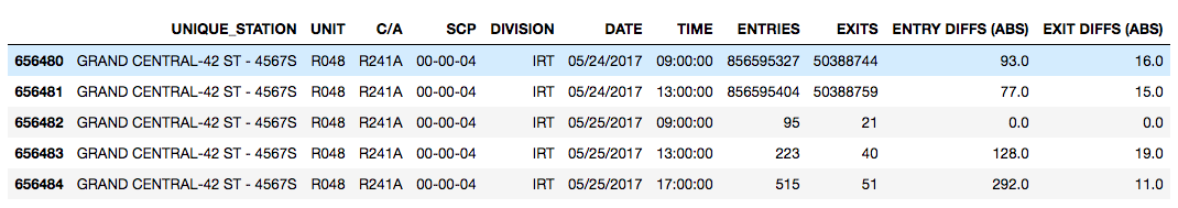
Filtered values are placed in two new columns named ENTRY DIFFS (ABS) and EXIT DIFFS (ABS). Note here how the value generated by this turnstile reset has been set to 0:

Calculating the Busiest Stations

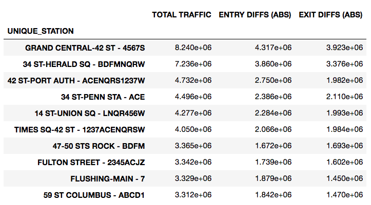
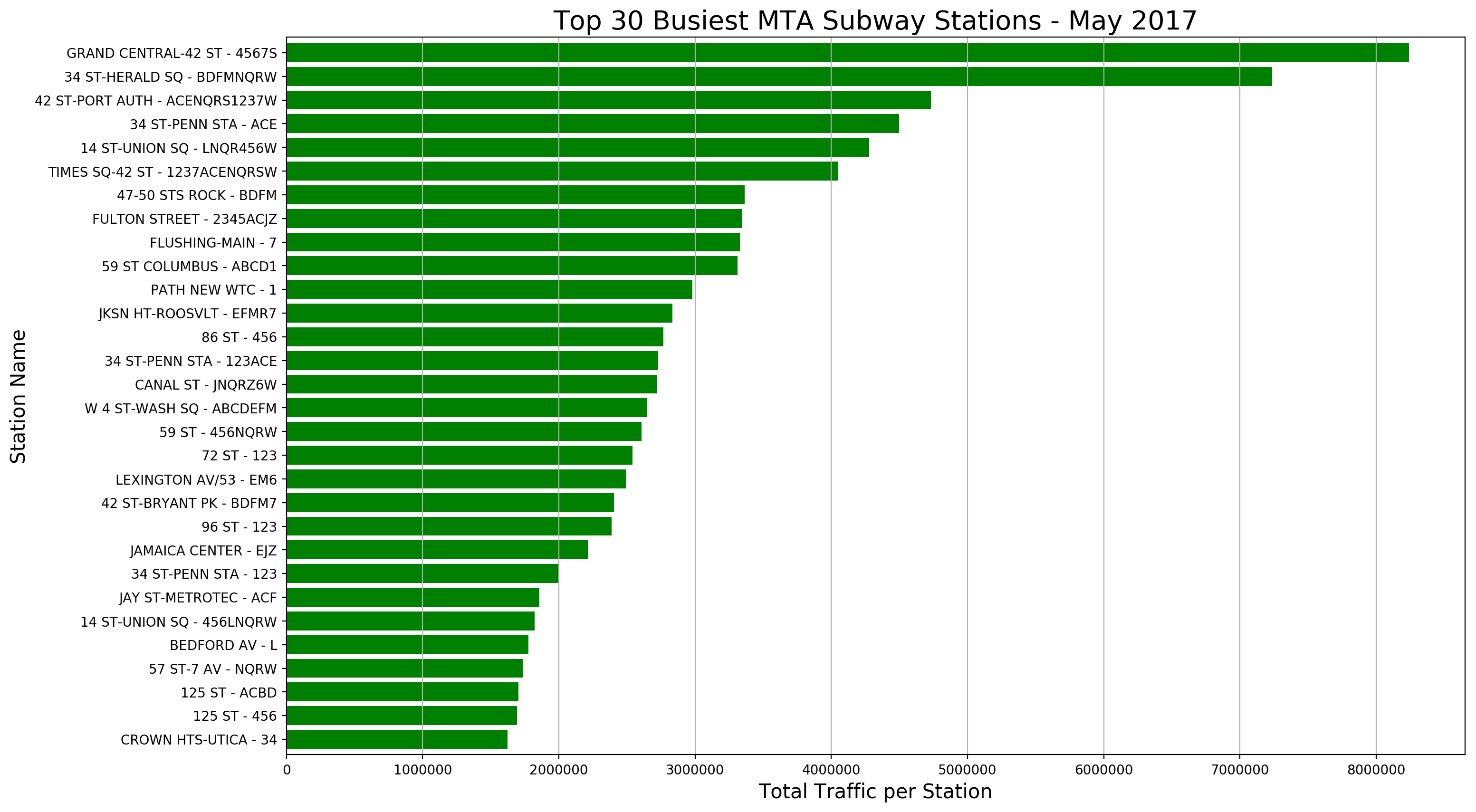
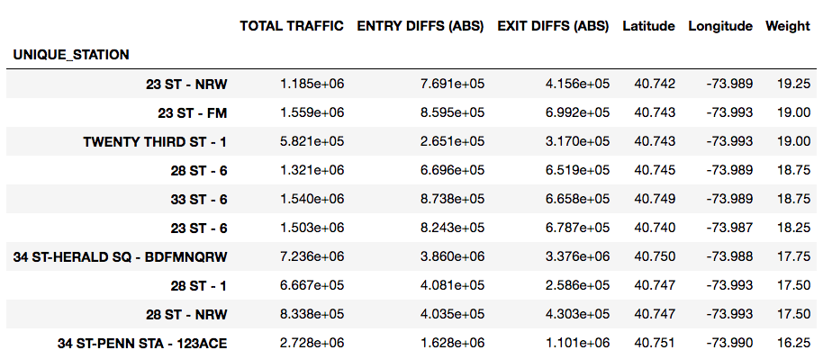
At this point, to calculate the most heavily-trafficked stations, we sum ENTRY DIFFS (ABS) and EXIT DIFFS (ABS) into a new column, TOTAL TRAFFIC, then group by UNIQUE_STATION, and look at the head:

We can also create a plot of the top 30 busiest stations:

This .groupby() dataframe of traffic per station is saved as a new dataframe for ease down the road.

Weighting Stations

Finding Locations

Now we need to weight stations based on their proximity to our list of relevant tech companies and colleges. First thing needed is exact locations. Using the Google Maps API, we can automate a search for each subway station (using the UNIQUE_STATION string, with station name and line) and company/college, then pull the latitude and longitude from the search result. (This search result is a formidable dictionary of lists and dictionaries, but a bit of parsing yields the proper series and keys and indices.)

Two main challengs appear here, beyond simply getting the search to work, First, many of the station names are abbreviated in the MTA database, and do not return a result. In my search function, I have it return a list of all queries for which there was no result, along with a dictionary of latitude and longitude (or NaN) for each station. For each station on this list, I attempt a more thorough renaming (e.g. HOYT-SCHER - ACG became HOYT-SCHERMERHORN - ACG), and then feed the renamed list back into the search function. A few passes, and all stations return results.

Next, after a little inspection, it becomes evident that the API is returning the same locations for multiple stations. This is immediately evident with all five 23rd St stations (CE, 1, F, NRW, 6), which are all listed as having the latitude and longitude of the 23rd St - NRW station. At this point, we turn to Stone Age tactics, look up the actual latitude and longitude on an MTA database of station information, and hard-code it into the location dictionary. When complete, we join this location dictionary to the new dataframe of traffic by station — a reasonably seamless operation, as the keys of the dictionary are the indices of the dataframe.

Determining Proximity Weights

To find the distance between stations and tech companies or colleges, we employ a function from the geopy.distance module called vincenty, which returns the distance between two points, in specified units, given two pairs of latitude and longitude measurements.

The more tech companies and colleges in direct proximity to any given station, the higher its value: we posit that the busiest station is of no value if the relevant traffic isn’t there. For each station-company/college distance, we assign a value, as such:

• 0-0.25 mi – 1 point
• 0.25-0.5 mi – 0.75 points
• 0.5-0.75 mi – 0.5 points
• 0.75-1 mi – 0.25 points
• Greater than 1 mi – 0 points

We assume that there are minimal cases where someone would elect to walk to a station more than a mile away, given the large chance of a more relevant option existing closer, thus the 0 for any distance greater than that. All points are added up per station, providing its proximity weight.

This is all achieved by feeding a weighting function to the .apply() method on the traffic dataframe, which allows us to perform the same operation on each row of the dataframe — or the data for each station, in this case. The function takes the latitude and longitude of each station, iterates through the latitude and longitude of each company/college, calculates the distance and then feeds that to another function that returns a point value, sums all points for the station, and returns the proximity weight as a number that we then feed into a new column.

Station Relevance

We assume that the stations we want to target are the ones with the most traffic and the highest proximity weight, thus the stations of greatest interest will fall in the upper right section of this scatterplot:

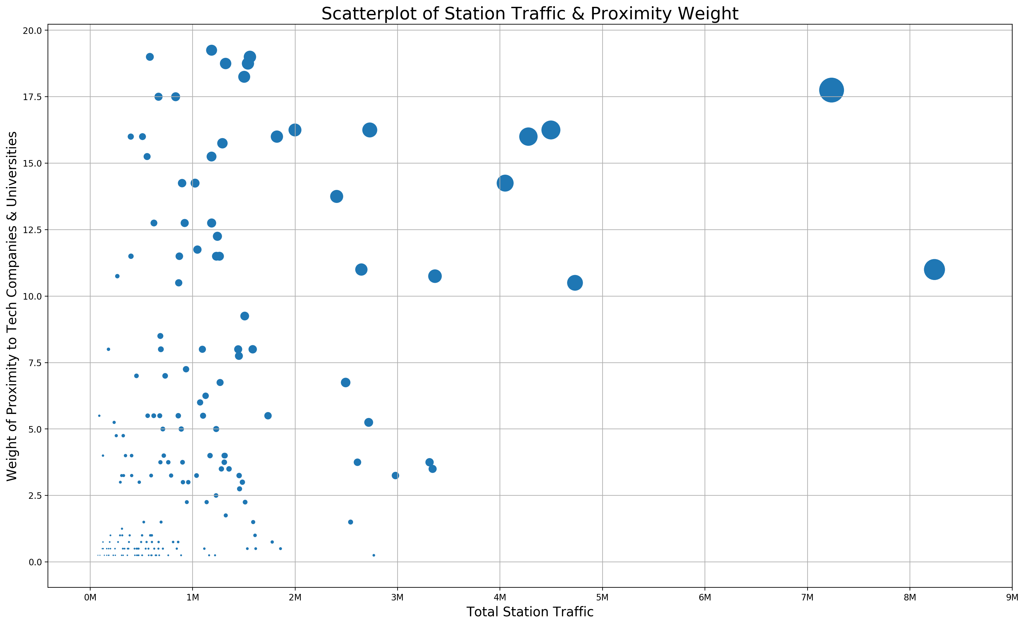
This value, we will call “relevance”, and calculate by multiplying the total traffic of a station by its proximity weight, then dividing by a scaling factor to put it into a reasonable range. Since the largest total traffic value is 8.24 million, and the largest proximity weight is 19.25, we choose 10 million as a scaling factor:

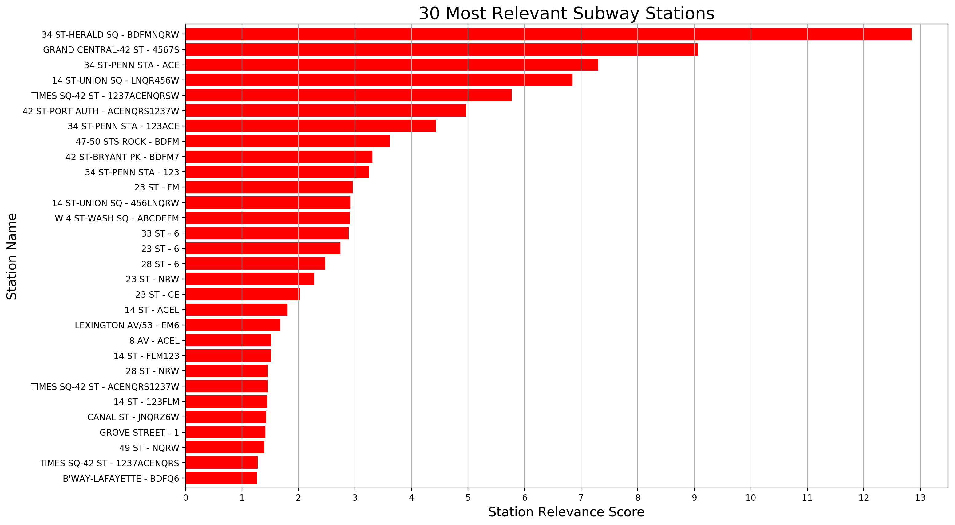
Relevance = (Traffic * Weight) / 1e7

Calculating relevance as a new column, we can then sort by it, and create a plot of the most relevant stations:

Conclusion/Recommendations

Not knowing the extent of our client’s promotional capabilities (e.g. number of street teams, cost of street teams, budget for promotion, etc.), we can’t advise exactly how many stations to cover or how long to cover them. What we can recommend is to start at the top of this list, and continue as far down as resources allow. We would also assume that since much of the value of a station is determined by its proximity to places of employement, the best time to canvas these stations would be when people are leaving the office and going home, somewhere in the 5pm-8pm range.

Other Thoughts

Clearly, the main focus of this project was to work with the turnstile data set in Pandas, to gain experience in exploring and cleaning a large dataset, and that objective was certainly met. I kept thinking throughout, though, that the total traffic of a station might be irrelevant in this situation, and that the quality of the traffic per station would be of utmost importance. High traffic may actually have diminishing returns, given a large flood of people focused only on getting down the stairs, onto the platform, and into the train. Of course, traffic needs to be present, but if there are numerous companies around a particular station, that station will have traffic. Were I only charged with addressing the question, I would focus on building a comprehensive list of relevant companies, perhaps from 100-500, and weighting stations based on proximity alone. I would also try to derive such a list from a pre-existing dataset, as opposed to building it manually.

I don’t completely trust the results of the Google Maps API either, and would want to review them further before standing by their complete accuracy in providing proximity weighting. Given the mishap with the 23rd St station, I wonder how many other stations were similarly affected, or if the right results were returned for all the companies and colleges. The current approach also doesn’t factor in the possibility of multiple offices or campuses per company. With more time, I would have tried to validate each location in some way, or figure out how to merge available subway location information with the turnstile data. Building a comprehensive list of company office addresses to search would be a more reliable way about it as well.